A coupled-oscillator image model, 6.1× smaller and ~5.8× faster.
Un-0 generates images by integrating a system of coupled oscillators. Its released CIFAR-10 model, cifar10/n4096, holds 19.4 million parameters and spends most of a sample stepping a dense oscillator-to-oscillator coupling. un0++ keeps that model's output quality and cuts its size and its runtime two independent ways that multiply: a precision change that routes the math onto the GPU's tensor cores with the same weights, and a structured replacement for the coupling that removes 6.1× of the parameters.
Written to be read cold. Every concept, model, and metric is explained where it appears, with the deeper mechanics behind the expandable panels and a glossary at the end. Every number was measured on the GPUs named in the footer.
Inference is running a finished model to produce output, as opposed to training it. It is the part that repeats for every image, so it sets the running cost. The work here reduces that cost without changing the pictures the model makes.
What is fixed. The starting point is Un-0's released cifar10/n4096 checkpoint (19.43M parameters), scored by the same quality metric Un-0 reports (clean-FID on CIFAR-10). One lever reuses those exact weights; the other trains a smaller model from scratch to the same quality. Both are measured against the model as it ships, on a data-center A100 and a smaller T4.
01 the model · generation by coupled oscillators
What Un-0 is, and where its time goes
Most image generators denoise or upsample. Un-0 treats a picture as the resting state of a field of coupled oscillators and integrates their dynamics until they settle.
Picture a runner on a circular track. Its position is an angle, its phase θ; left alone it circles at its own natural frequency ω. Now connect many such runners so each feels a pull toward the others. That pull is the Kuramoto model: every pair (i, j) interacts through sin(θj − θi), which speeds a lagging phase up and slows a leading one down. With enough coupling the phases lock together, a behaviour seen in firefly flashing and pacemaker cells.
Un-0 uses 4,096 oscillators (that is what n4096 means). Instead of one uniform pull toward the group average, it gives every pair its own learned coupling strength Kij. Chosen well, those strengths steer the 4,096 phases into a pattern that decodes to a specific 32×32 image. The panel below shows the plain version, all phases pulling toward one average, so the mechanism is visible.
The dynamics Un-0 integrates for each oscillator i:
To draw an image the model starts the phases from noise and advances this equation for 10 solver steps (a plain Euler integrator), then decodes the settled phases to pixels. The generation is deterministic given the seed. The full batch of 1,024 images is integrated together on the GPU.
The learned coupling K is a dense 4,096 × 4,096 matrix, one number for every ordered pair of oscillators. That single matrix is 16.8M of the model's 19.4M parameters, and evaluating the sum above once costs on the order of n² = 16.8 million multiply-adds. Because the sum runs every solver step, the dense coupling dominates both the model's size and its per-step compute. Everything un0++ does targets that n² term.
Why the coupling can be replaced without touching the physics
The velocity equation looks like it needs the full matrix K, but expand it with the angle-difference identity: sin(θj−θi) = sinθj·cosθi − cosθj·sinθi. Substituting, the whole coupling term reduces to cosθi·(K·sinθ) − sinθi·(K·cosθ). The matrix K only ever appears applied to two vectors, sinθ and cosθ.
So K is used purely as a linear operator, never as a table of numbers you read individually. Any object that computes K·v for a vector v can stand in for it, including a structured operator with far fewer parameters and a faster matrix-vector product. That single fact is what makes the compression in section 03 possible without changing the oscillator dynamics. The diagonal of K is irrelevant here, since the j=i term carries sin(0)=0.
clean-FID (Fréchet Inception Distance) scores image quality. It passes both real CIFAR-10 images and generated ones through a fixed image-recognition network (Inception), then measures the distance between the two sets of features. Lower is closer to real; a difference under ~0.1 is within seed-to-seed noise. "clean-FID" is a standardized implementation that removes resizing artifacts, and it is the exact metric Un-0 reports. All FID here is scored on 50,000 class-balanced samples.
Throughput is images generated per second for a full batch; higher is better. Latency is the wall-clock time for one sample() call; lower is better. The two move together here because a whole batch is generated in one call. CIFAR-10 is the benchmark dataset: 60,000 color images at 32×32 pixels across 10 classes.
02 lever one · the tensor-core inference path
Free speed from the released weights
The first lever changes no weights and retrains nothing. It changes the number format the math runs in, which moves the work onto hardware units that sit idle by default.
A modern NVIDIA GPU has two kinds of math unit. The general-purpose cores run 32-bit floating point (fp32), the default, accurate and comparatively slow for matrix multiplies. Alongside them sit tensor cores, units built only for matrix multiply-accumulate and several times faster, but they run in reduced precision. Un-0 as shipped computes in fp32, so the tensor cores go unused.
Three formats reach them. TF32 keeps fp32's numeric range but rounds the mantissa so fp32 matmuls dispatch to the tensor cores, a near-invisible accuracy change turned on with one flag. bf16 and fp16 are 16-bit floats that halve the data moved and run the tensor cores at full rate: bf16 (wide range, used on the A100) and fp16 (used on the T4). Mixed precision (autocast) is the policy that runs each operation in the fastest format that is safe for it, keeping sensitive reductions in fp32 while the heavy matmuls go 16-bit.
Turning on TF32 plus bf16/fp16 autocast, on the released dense model, same weights, no retraining:
A100 · dense weights unchanged
Why this needs no hand-written GPU kernel
A kernel is a single program the GPU runs. There are two separate things one could call a kernel here, and only one is doing the work. The tensor-core path turns on TF32 and 16-bit autocast so PyTorch dispatches to the vendor's already-optimized matrix kernels (cuBLAS, cuDNN), and torch.compile fuses the elementwise glue around them. No new kernel is authored; the work is routed to the right existing ones.
A hand-written kernel is the separate question of whether custom code on top adds anything, taken up in section 04. On this model it does not, materially, because the compiler is already a strong baseline. The banked speedup here comes entirely from precision plus the compiler, not from bespoke code.
03 lever two · Monarch-structured compression
Removing the coupling's quadratic cost
The second lever is independent of the first. It rebuilds the model so the dense 4,096×4,096 coupling, the object holding 16.8M of the 19.4M parameters, is replaced by a structured operator with a fast matrix-vector product, then trains that model from scratch to the same quality.
A dense n×n matrix stores every entry and costs n² to apply. A Monarch matrix approximates that operator as a short product of two cheap pieces: a block-diagonal matmul (split the n values into √n groups and mix within each group only) followed by a fixed block-to-element transpose (a reshuffle that lets the next block-diagonal step mix across the earlier groups). Two such stages let information reach anywhere, at a cost that grows like n1.5 instead of n².
For n=4096 the √n groups are 64 blocks of 64. Each Monarch factor is 64×64×64 = 262,144 numbers. A depth-2 product is two factors, 0.52M parameters, against the dense coupling's 16.8M. Same role in the dynamics, 32× fewer numbers, and a sub-quadratic apply.
The swap is opt-in by config. The dense code path is left byte-identical, so the released model reproduces exactly; a monarch flag routes the sin/cos vectors through the structured operator instead. From Un-0's dynamics, the coupling collapses like this:
the coupling, at matched quality
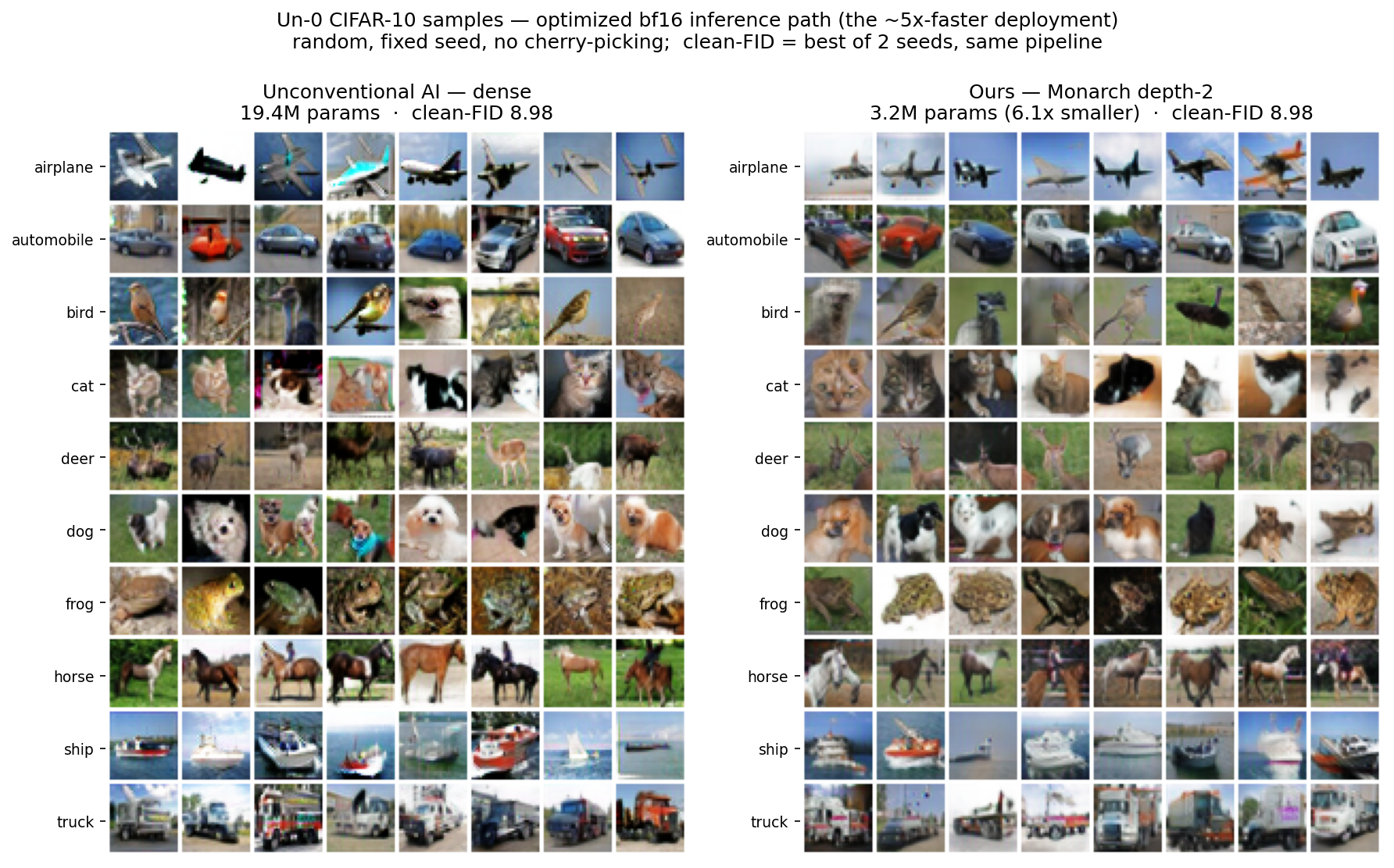
Quality holds at the smaller size. Two seeds per model; "min" is the better seed, reported because a single FID draw carries noise.
| Model | Params | Compression | clean-FID fp32 (min) | clean-FID bf16 (min) |
|---|---|---|---|---|
| Released dense cifar10/n4096 | 19.43M | 1.0× | 8.88 | 8.98 |
| Monarch depth-2 (featured) | 3.18M | 6.1× | 8.93 | 8.98 |
| Monarch depth-3 + low-rank (variant) | 3.97M | 4.9× | 9.00 | — |
Independent re-measurement of the released checkpoint lands at 8.88–8.89 fp32, reproducing Un-0's published figures (8.86 repo, 8.76 blog) within seed noise, which confirms the pipeline is on their exact ruler. On the bf16 deployment path the 6.1×-smaller model and the full model are dead even at 8.98.
The two-line change, and the low-rank residual that closes the gap
The whole contribution is two edits to the model. Construction swaps the dense n×n parameter for the Monarch operator. Forward routes sinθ and cosθ through that operator and recombines them with ω + cosθ·(K·sinθ) − sinθ·(K·cosθ), the same angle-difference form from section 01. No dense matrix is ever built.
Block-local Monarch factors mix only within √n-sized blocks per stage. Some couplings are global and rank-concentrated, which pure Monarch misses. An optional low-rank residual, (x·V)·Uᵀ, adds a cheap global channel of rank r at O(n·r) cost. Its output weight U is initialized to zero, so the model starts as pure Monarch and grows the global path only as training demands. Fitting a fixed trained dense matrix with either structure alone fails badly (over 96% error), but co-training Monarch and low-rank from scratch lets each cover the other's blind spot.
The depth-3 variant adds a third factor and a rank-64 residual, 3.97M parameters. Its extra capacity did not buy quality (9.00 vs depth-2's 8.93, min FID), so the smallest structured model is the one to ship.
Why 6.1× fewer parameters is not 6.1× faster on its own
Cutting parameters cuts memory and math, but wall-clock also depends on how the work maps to the GPU. A single dense 4,096×4,096 matmul is one large, tensor-core-friendly operation. The Monarch operator is many small 64×64 block matmuls, each a separate GPU launch, and small matmuls leave the tensor cores underfed. So the 6.1× parameter cut is worth about 1.6× wall-clock on its own (A100, batch 1024: 102 ms dense to 65 ms depth-2, both fp32). The larger end-to-end win comes from stacking this on the tensor-core path, section 04.
04 stacked · end-to-end and the floor
Both levers together, and how close to the floor
The precision path and the compression are independent, so they multiply. Each row below is the same generation task at batch 1024; the bar is images per second, the tail is the speedup over the model as it ships.
A100 (data-center GPU, 80 GB)
T4 (smaller inference GPU, 16 GB)
A100 batch-1024 sample · was 102 ms
The next question is whether a hand-written kernel adds more. Profiling the 17.7 ms sample end-to-end shows it does not, materially.
Where the ~18 ms actually go, and why a custom kernel is capped near 1.1×
A profiler over the bf16 sample (batch 1024) splits the wall-clock cleanly. Of 18.4 ms, about 11.9 ms is the GPU doing math and about 6.5 ms (~35%) is host-side idle: the Python solver loop launching each step's kernels one at a time while the GPU waits between them. That 35% is the single largest block, and no per-step kernel can touch it.
Inside the GPU-busy time, the coupling matmul is still the biggest slice at 23%, because Monarch's small block matmuls lower to a memory-bound matrix-vector product (a GEMV) that leaves the tensor cores idle. A hand-written Triton kernel fixes exactly that, folding both Monarch factors and the transpose into two tensor-core launches. It is correct (bit-exact in fp32) and runs 1.34× faster than the compiler on the coupling in bf16. But the coupling is 23% of compute, so by Amdahl's law that is worth at most ~1.1× end-to-end, and it leaves the 35% host idle untouched.
The negative results: a wider kernel loses to the compiler, and CUDA-graph capture fails
Widening the hand-written kernel to the whole velocity step (sin/cos, both Monarch factors, the scale, the recombine) makes it slower than torch.compile: 0.69× in bf16. The compiler already computes sin and cos once and reuses them, folds the recombine into the matmul epilogues, and picks good tile sizes; the hand-written version recomputes trig and its fixed tiles do not match. The coupling-only win exists precisely because it attacks the one primitive (GEMV) the compiler lowers badly; give the compiler back the surrounding elementwise work and it wins.
Attacking the 35% host idle means replaying the whole 10-step rollout as one captured GPU sequence. Managed CUDA graphs (reduce-overhead) give 0.96×, no help, and a manual full-rollout capture fails outright (cudaErrorStreamCaptureInvalidated): the model already runs torch.compile internally with its own graph trees, and an outer capture cannot wrap them. Recovering that time needs a solver rewrite (a single fixed-step, static-shape, graph-safe loop), not a kernel. The one untested lever is algorithmic: fewer solver steps (10 to 6–7) would give ~1.4–1.6× if an FID re-check confirms quality holds.
The coupling was the whole cost
The dense 4,096² matrix is 16.8M of 19.4M params and O(n²) per step. Monarch cuts it to 0.52M at O(n1.5), same role in the dynamics.
Tensor cores are free speed
TF32 + 16-bit autocast on the released weights, no retraining: 4.82× on A100, 3.36× on T4 at batch 1024. The default fp32 path never touches them.
Quality holds at 6.1× smaller
depth-2 (3.18M) matches dense (19.43M) at clean-FID 8.98 on the bf16 path, and 8.93 vs 8.88 in fp32. bf16 generation costs under 0.1 FID.
Compression is 6.1× params, ~1.6× speed
Many small Monarch matmuls are launch-bound, so the parameter cut gives ~1.6× wall-clock alone. Stacked on the tensor-core path it reaches 5.77× end-to-end.
Close to the floor
~35% of the 18 ms A100 sample is host-side ODE-loop idle, not GPU math. The coupling is 23% of GPU time. A custom kernel adds ~1.1× at most.
The compiler is the baseline
A fused whole-step Triton kernel runs 0.69×, slower than torch.compile. The only kernel win is the isolated coupling matmul, 1.34× in bf16, a GEMV the compiler lowers badly.
05 glossary
Every term and entity, defined
- Un-0
- An open image-generation model that draws pictures by integrating coupled-oscillator dynamics. cifar10/n4096 is its released 19.4M-parameter CIFAR-10 model, the starting point here.
- Kuramoto oscillator
- A phase that circles at its own natural frequency and feels a pull toward other phases through a sine of their difference. The classic model of synchronization (fireflies, pacemaker cells).
- Phase (θ) / natural frequency (ω)
- An oscillator's angle on its circle, and the rate it would circle uncoupled. Un-0's images are patterns of settled phases.
- Coupling matrix (K)
- The learned strength of every oscillator pair's interaction. In Un-0 a dense 4,096×4,096 matrix, 16.8M of the model's 19.4M parameters.
- Order parameter
- A single number from 0 to 1 measuring how aligned the phases are. 0 is scattered, 1 is fully synchronized.
- ODE solver / Euler step
- The method that advances the dynamics in discrete time. Un-0 samples with 10 plain Euler steps per image.
- CIFAR-10
- A benchmark dataset: 60,000 color images at 32×32 pixels across 10 classes. The task Un-0 is trained on.
- Parameter count
- The number of learned weights in a model. Sets memory footprint and part of the compute. 19.43M dense, 3.18M for the featured compressed model.
- FID / clean-FID
- Fréchet Inception Distance: the distance between Inception features of real and generated images. Lower is better. clean-FID is the standardized, resize-artifact-free implementation Un-0 reports.
- Inception
- The fixed image-recognition network whose internal features FID compares. Not trained here; used only as a measuring stick.
- Throughput vs latency
- Images per second for a full batch (higher better) versus wall-clock for one call (lower better). They track together here since a batch is one call.
- Batch
- How many images are generated in one call. Numbers here are batch 1024 and batch 256.
- Tensor core
- A GPU unit built only for matrix multiply-accumulate, several times faster than the general cores but running in reduced precision.
- fp32
- 32-bit floating point, the accurate default. Un-0 ships computing in fp32, which never reaches the tensor cores.
- TF32
- A tensor-core format keeping fp32's range with a shorter mantissa, so fp32 matmuls run on tensor cores with a near-invisible accuracy change.
- bf16 / fp16
- 16-bit floats that halve data moved and run tensor cores at full rate. bf16 (wide range) on the A100, fp16 on the T4.
- Mixed precision / autocast
- Running each operation in the fastest safe format, heavy matmuls in 16-bit, sensitive reductions in fp32.
- Monarch matrix
- A structured operator that approximates a dense matrix as a block-diagonal matmul plus a block-to-element transpose, applied at O(n1.5) cost instead of O(n²).
- Block-diagonal
- A matrix that mixes values only within √n-sized groups. The cheap core of a Monarch factor; the transpose lets a second one mix across groups.
- Low-rank residual
- A cheap global channel (x·V)·Uᵀ added to Monarch to capture couplings its blocks miss. Zero-initialized, so it grows only as training needs it.
- Sub-quadratic / O(n²) vs O(n1.5)
- How cost scales with oscillator count. Dense coupling is quadratic; Monarch is sub-quadratic, the reason the parameters collapse.
- GEMM / GEMV
- Matrix-matrix vs matrix-vector multiply. GEMM feeds tensor cores well; GEMV is memory-bound and leaves them idle. Monarch's small blocks lower to GEMV.
- Kernel
- A single program the GPU runs. The tensor-core path routes work to the vendor's kernels; a hand-written kernel is custom code, studied and found to add little here.
- Launch-bound
- Limited by how fast the CPU issues GPU work, not by GPU math. Many small Monarch matmuls are launch-bound, which is why 6.1× fewer params is only ~1.6× faster.
- torch.compile / Inductor / Triton
- PyTorch's compiler, its GPU backend, and the language for writing GPU kernels. The compiler fuses the elementwise work and is a strong baseline here.
- CUDA graph
- A recording of a sequence of GPU operations replayed as one launch. Attempted to remove the host idle; capture fails against the model's internal compiled graph trees.
- Amdahl's law
- A speedup on one part is capped by that part's share of the whole. The coupling is 23% of compute, so a coupling-only kernel tops out near 1.1× end-to-end.
- T4 / A100
- Two NVIDIA GPUs. T4: smaller inference card (16 GB, fp16 tensor cores). A100: data-center card (80 GB, TF32/bf16 tensor cores) used for training, FID, and the kernel study.
- Distillation
- Training a small model to copy a larger one's outputs. Not used here; the compressed model is trained from scratch, so parity is on clean-FID, not per-image match.